1. Linear classifiers – Support Vector Machines for Credit Scoring

The main task of the credit scoring is simple: build a model, which will be able to distinguish between a good creditor and a bad one. Or put in other words: take the past credit data set and use them to learn the rules generally applicable for the future discrimination between the two creditor classes, with minimal number of mistakes both in false positives and false negatives.

The task to assign an observation to its respective class is called Classification.

Since for the purpose of the credit scoring, there are only two possible categories (e.g. 0 = good creditor, 1 = bad creditor), this specific setting of the classification is referred as Binary classification. Apart from the credit scoring, the binary classification has a wide variety of applications; no wonder there have been several different approaches developed in the literature.

No fewer than two scientific fields are intersecting in this task: Statistics and Machine Learning.¹ While the methods and scope of these fields may be different in general, it is practically impossible to draw a clear line between them in the context of the data classification problem.²

Machine Learning accents the ability to make a correct prediction, while Statistics accents the ability to describe the relationships among the model variables and to quantify the contribution of each one of them.

The classification problem is sometimes called supervised learning, because the method operates under supervision [58]. As mentioned above, the learning process in the credit scoring usually begins with some historical, labelled³ observations. These observations are often referred as the training set.

The goal of the supervised learning is to derive a mapping (function) which not only can correctly describe the data in the training set, but more importantly is able to generalize from the training set to the unobserved situations.
Since the main application of the classifier models is the prediction, the generalization ability of the learning algorithms are by far the most important property that distinguishes a good classifier from the bad one. [28]

The function derived from the supervised learning introduces a border between two classes – we say it forms a decision boundary or decision surface. Depending on the shape of this decision boundary we distinguish linear classifiers and non-linear classifiers. The linear classifiers represent a wide family of algorithms, whose common characteristic is that the decision is based on the linear combination of the input variables [51, p. 30]. All the classifiers described and used in this thesis, namely Logistic regression and Support vector machines, can be regarded as members of this wide family.

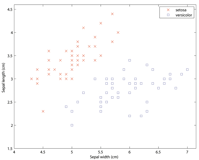
Fisher in his classic paper [23] introduced his linear discriminant, which was probably the first linear classifier. The Iris Data set [2], published in the same paper to demonstrate the power of his linear discriminant, became eventually the most cited classification data set, used widely for educational and explanation purposes. A subset of this data set is presented at Figure 1. It demonstrates a simple example of the binary classification problem with 2 explanatory variables and 100 observations. The goal of the classification is to draw a line that could serve as a borderline between the two different classes. Since the data are clearly linearly separable, it does not appear to be much a challenging task.

**Figure 1.** An example of a linearly separable binary classification problem based on the Fisher Iris Data (citation and detail in the text). In principle there is an infinite number of lines that could serve as a decision boundary perfectly separating the two classes.

Definition 1.1. Two subsets X and Y of $\mathbb{R}^d$ are said to be linearly separable if there exists a hyperplane of $\mathbb{R}^d$ such that the elements of X and those of Y lie on opposite sides of it. [20]

In principle, there is an infinite number of lines capable of performing this task. However, we can intuitively feel, that not all of them are equally good at it and that there are lines which accomplish this task better than others. Before we define what “good” and “better” means in this context, let’s have a closer look at the Iris dataset.

Geometric interpretation of the data points

As already mentioned, there are 100 data points (observations) with 2 input variables (sepal width and sepal length in cm) and one binary class variable (setosa/versicolor). The mere fact that, in Figure 1, we chose to display the data set as a two-dimensional scatter plot implicitly assumes, that each property can be regarded as a dimension in a coordinate system. Each data point can therefore be interpreted geometrically, as a point in a coordinate system.

This can be taken even further, though. Each data point can be visualised as a vector rooted in the origin of a coordinate system.⁴ [28, p. 33]

Definition 1.2. Vector is a directed line segment, that has both length and direction. [40, p. 355]

Definition 1.3. Given the components of vector, $\vct{a} = (a_1,a_2,\dots,a_n)$ , the length or norm of a vector $\vct{a}$ , written as $\|\vct{a}\|$ , is defined by:

(1) $\begin{equation*} \|\vct{a}\| = \sqrt{a_1^2 + a_2^2 + \dots + a_n^2} \end{equation*}$

The geometric interpretation of vectors is conceptually very advantageous. Effectively, we have converted our data universe into a vector space. By allowing this, we can compute new objects using algebraic vector operations. More, it is possible to calculate the dot products of two vectors which can then serve as a measure of similarity between two observations.⁵ [28, p. 34]

Definition 1.4. Given two vectors $\vct{a}$ and $\vct{b}$ from $\mathbb{R}$ the dot product or inner product of $\bf{a} \cdot \bf{b}$ is:

(2) $\begin{equation*} \vct{a}\cdot\vct{b} = \sum_{i=1}^n a_ib_i\\ \end{equation*}$

Remark 1.1. There is a relation between the length of a vector and the dot product of a vector with itself:

(3) $\begin{equation*} \| \vct{a} \| = \sqrt{\vct{a} \cdot \vct{a}} \end{equation*}$

To construct a decision boundary in this example, one has to find a line such that it will separate one class of the training data set from the other one.

Definition 1.5. A set of points $(x_1,x_2) \in \mathbb{R}^2$ satisfying equation

(4) $\begin{equation*} w_1x_1 + w_2x_2 + b = 0 \end{equation*}$

is called a line.

Remark 1.2. Note that we may express the equation (4) in the vector form as

(5) $\begin{equation*} \vct{w} \cdot \vct{x} + b = 0 \end{equation*}$

The beauty of the vector form (5) lies in the fact, that it is valid in general for any number of dimensions, i.e. for the data sets with more than just two explanatory variables.

In the three-dimensional settings, if we let $\vct{w}, \vct{x} \in \mathbb{R}^3$ , that is $\vct{w} = (w_1, w_2, w_3)$ and $\vct{x} = (x_1, x_2, x_3)$ , the equation (5) will not change and the subset of all points satisfying this equation is called a plane.

More generally, in n-dimensional space, we call the subset of all points satisfying (5) a hyperplane. A hyperplane is an affine subspace of dimension n-1 which divides the space into two half spaces. [14, p. 10]

The notation $\vct{w}$ and $b$ was chosen with an agreement of the majority of the SVM literature; $\vct{w}$ standing for weight vector and $b$ for bias, both terms coming originally from the perceptron research, which has historically much common with the support vector machines [14, p. 10]. The statistics literature usually refers both as parameters.

Classification formalized

The classification problem can be formalized as follows:

Let the dot product space $\mathbb{R}^n$ be the data universe with vectors $\boldsymbol{x} \in \mathbb{R}^n$ as objects
Let $S$ be a sample set such that $S \subset \mathbb{R}^n$
Let $f : \mathbb{R}^n \to \{+1,-1\}$ be the target function
Let $D = \{ ( \vct{x}, y )\ |\ \vct{x} \in S \land y = f(\boldsymbol{x}) \}$ be the training set

Find a function $\hat{f} : \mathbb{R}^n \to \{+1,-1\}$ using $D$ such that

(6) $\begin{equation*} \hat{f}(\vct{x}) \approx f(\vct{x}) \end{equation*}$

for all $\vct{x} \in \mathbb{R}^n$ . Depending on $n$ , we construct line, plane or hyperplane, that separates classes $+1$ and $-1$ as best as possible. The resulting linear decision surface is then used to assign new objects to the classes. [55, p. 1], [28, p. 50]

Vectors $\vct{x}$ are usually referred in the literature as patterns, cases, instances or observations; values $y$ are called labels, targets or outputs. [55, p. 1]

As already mentioned, we call this problem binary classification problem. It is caused by the fact, that the output domain $Y = \{ +1, -1 \}$ consists of two elements. In more general cases, for $Y = \{ 1,2,\dots,m \}$ , the task is called m-class classification. For $Y \subseteq \mathbb{R}$ we speak about regression. [14, p. 11] While the support vector machines can also be used, with some simple modifications, for the m-class classification and for the regression, these modifications hardly have any use in the context of the credit scoring and are not a subject for this thesis.

Having the normal vector $\vct{w}$ and bias $b$ from (5), the task to classify new observation $\vct{a}$ is quite simple. Should the observation belong to the $+1$ class, the point will lie above the decision surface and the value of (5) will be positive. On the contrary, all observations belonging to the $-1$ class will lie below the decision surface and the value of (5) will be negative. The decision function $\hat{f}$ can be constructed as follows [28, p. 50-51]

(7) $\begin{equation*} \hat{f}(\vct{x}) = \begin{cases} +1 & \text{if $\vct{w} \cdot \vct{x} + b \geq 0$}\\ -1 & \text{if $\vct{w} \cdot \vct{x} + b < 0$} \end{cases} \end{equation*}$

That is, by defining the sign function for all $k \in \mathbb{R}$ as

(8) $\begin{equation*} sgn(k) = \begin{cases} +1 & \text{if $k \geq 0$}\\ -1 & \text{if $k < 0$} \end{cases} \end{equation*}$

the linear decision function for $\vct{w}, \vct{x} \in \mathbb{R}^n$ , $b \in \mathbb{R}$ can be constructed as

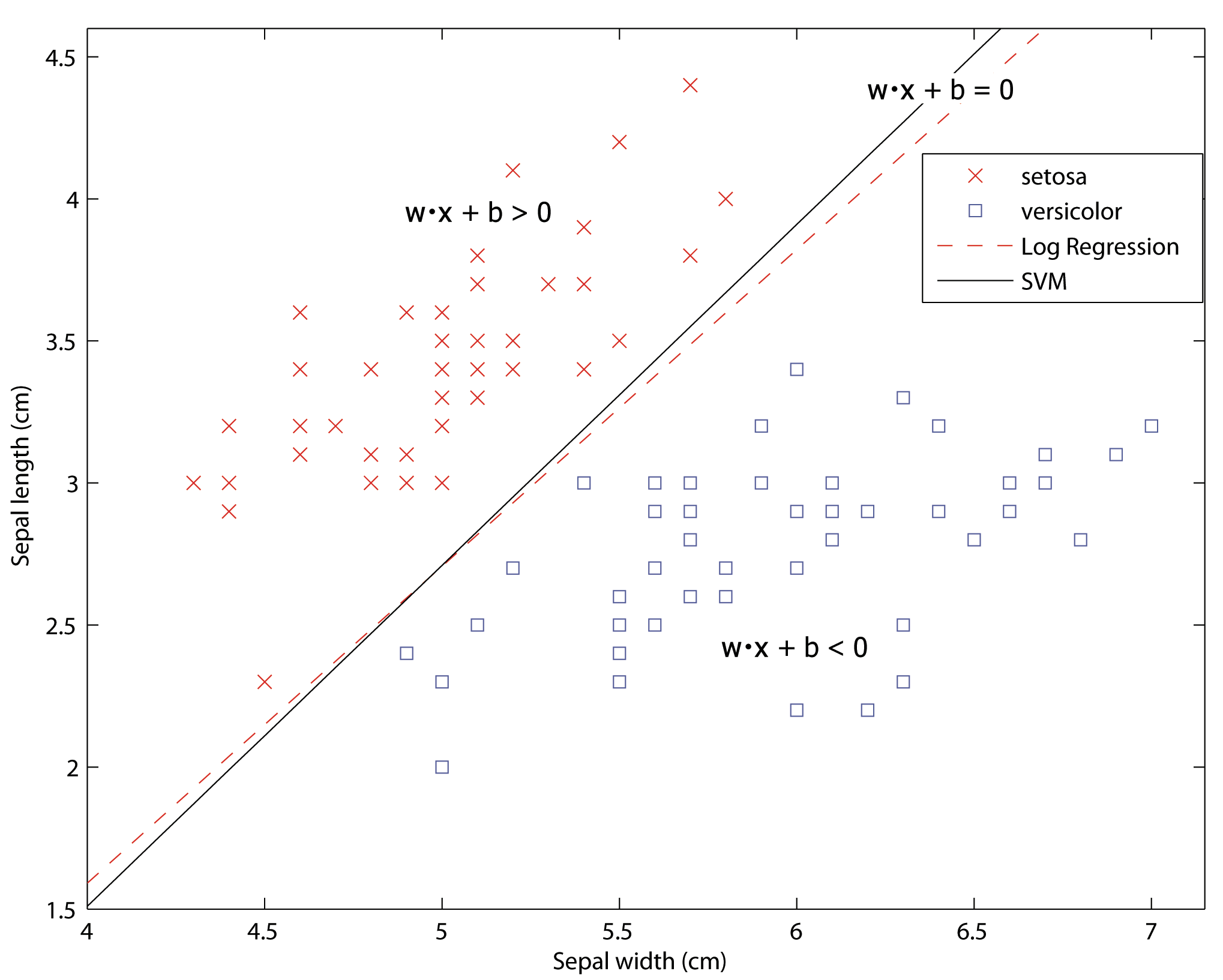
(9) $\begin{equation*} \hat{f}(\vct{x}) = sgn( \vct{w} \cdot \vct{x} + b ) \end{equation*}$

The situation is clearly demonstrated in Figure 2.

The key problem lies in the determination of the appropriate weight vector $\vct{w}$ and bias $b$ . There are basically two approaches to this job.

The generative learning aims to learn the joint probability distribution over all variables within a problem domain (inputs $x$ and outputs $y$ ) and then uses the Bayes rule to calculate the conditional distribution $p(y|x)$ to make its prediction. Methods like naive Bayes classifier, Fisher’s discriminant⁶, hidden Markov models, mixtures of experts, sigmoidal belief networks, Bayesian networks and Markov random fields belong to this class of models. [38]

The discriminative learning does not attempt to model the underlying probability distributions of the variables and aims only to optimize a mapping from the inputs to the desired outputs, i.e. the model learns the conditional probability distribution $p(y|x)$ directly. These methods include perceptron, traditional neural networks, logistic regression and support vector machines. [38]

Discriminative models are almost always to be preferred in the classification problem. [47]

All these methods generate a linear decision boundary. That is, the boundary between the classes in the classification problem can be expressed in the form of the equation (5).

For example, the first and simplest linear classifier, the aforementioned Fisher’s discriminant, attempts to find the hyperplane $(\vct{w}, b)$ on which the projection of the training data is maximally separated. That is to maximize the cost function

(10) $\begin{equation*} F = \frac{(m_+ - m_-)^2}{\sigma_+^2 + \sigma_-^2} \end{equation*}$

where $m_i$ is the mean and $\sigma_i$ is the standard deviation of the projection of the positive and negative observations. [14, p. 20] The decision boundary is then perpendicular to this hyperplane.

Logistic regression

Although its name would indicate otherwise, the logistic regression also belongs to the linear classifiers. Thanks to its very good performance and a long history of successful utilization, it is widely acknowledged that the logistic regression sets the standard against which other classifications methods are to be compared.⁷ [22] This thesis will not be an exception and it also uses the logistic regression as an etalon.

Unlike the classical linear regression where the response variable can attain any real number, the logistic regression builds a linear model based on a transformed target variable that can attain only values in the interval between zero and one [58]. Thus the transformed target variable can be interpreted as a probability of belonging to the specific class. For binary classification problem, the model is especially simple, comprising just single linear function [33]

(11) $\begin{equation*} \log \frac{P(Y=+1\ |\ X=\vct{x})}{P(Y=-1\ |\ X=\vct{x})} = \vct{w} \cdot \vct{x} + b \end{equation*}$

The maximum likelihood estimation (MLE) method is usually used to find the parameters $\vct{w}$ and $b$ , using the conditional likelihood of Y given the X. [33]

The left-hand side of (11) is called the log-odds ratio. Note, that in the situation when both probabilities, the one in the numerator as well as the one in the denominator, will be equal to 0.5, the log-odds ratio is zero. The equation will then simplify to (5). This is the equation describing the decision boundary in the logistic regression model; the set of points where the logistic regression is indecisive.

The difference in performance among the various linear classifiers arises from its different distribution assumptions or from the method used to the estimation of the parameters of the decision boundary $(\vct{w},b)$ . When we return to the geometrical interpretation of the input data, we can realize, that:

If established on reasonable assumptions, the boundary lines generated by different linear classifiers should be quite similar. An example of two decision boundaries on our example data set is presented in the Figure 2.
There is an upper bound to the performance of ANY linear classifier. In every binary classification problem, there exists a single line that best separates the two classes of data.

The reason, why some classifiers systematically outperform others in applications using the real data sets, depends on 3 key points. How well does the classifier handle:

the linearly inseparable data.
the random noise in the data and the outliers.
the non-linear relationships in the data.

As will be shown in the next chapter, the strength of the Support vector machines when compared to other linear classifiers lies in the fact that (1) it can separate linearly inseparable data, (2) it is almost immune against outliers, (3) it can fit non-linear data thanks to the technique generally referred as Kernel trick. The logistic regression, for comparison, lacks the last ability.

**Figure 2.** The sample data set with two possible linear decision functions – one obtained with the logistic regression, the second one with the support vector machines. Although the lines are not identical, they both could be regarded as satisfactory models to classify the iris flowers. It can be proved from the Vapnik-Chervonenkis theory that the decision surface obtained with the support vector machines is the optimal linear classifier under the condition that “optimal” is defined in terms of structure risk minimization.

Footnotes

¹ being part of a more general Computer Science field

² Consider for example the Logistic Regression, which is frequently used for classification. Logistic regression is widely considered to be a statistical tool and is still a standard performance benchmark for the credit scoring in the real-life banking [16]. On the other hand, Support Vector Machines (SVMs), which are the main topic of this thesis, are commonly referred as a machine learning tool. Yet they are actually very similar to each other: they both have a same goal and purpose and they both can be expressed as a hyperplane separating the space into two subspaces. The main practical difference between them lies in the terminology. Due to the key focus of my thesis, I will prefer the machine learning terminology, where appropriate.

³ i.e. we know, whether the loan applicant turned to be good or bad

⁴ (0,0) in this case

⁵ The dot product of two vectors computes a single scalar value, zero for orthogonal vectors, which can be interpreted as no similarity at all.

⁶ Also called as Linear discriminant analysis

⁷ This opinion, however, has recently been challenged in [42]. Other, more powerful classifiers were proposed as a norm for the performance comparison in future research instead.

Geometric interpretation of the data points

Classification formalized

Logistic regression

Footnotes

Leave a Reply Cancel reply