3. Model bulding – Support Vector Machines for Credit Scoring

In this chapter, some practical issues that need to be addressed when one builds a credit scoring model (or any other classification model) are discussed. While some of these issues are rather general and not solely limited to the support vector machines, the text was adjusted to the fact, that SVM will be my primary training algorithm in the practical part of this thesis.

Data preprocessing

Categorical variables

Support vector machines assume that each input observation is represented as a vector of real numbers. In some instances, and this is true especially for the credit risk applications, many features are not real numbers. They are either ordinal or categorical variables (e.g. education, gender, home ownership, $\dots$ ). Hence for the use of SVM algorithm, these variables need to be transformed into numerical ones.

One common approach is to express $r$ -category variable as a zeros-one vector of length $r$ . Thus for example gender {male, female} can be represented as (1,0) and (0,1), respectively. The increased number of attributes should not negatively affect the performance of the SVM. [35]

In fact, there is one dimension redundant in this approach. Merely $(r-1)$ -dimensional vector of zeros and ones is sufficient to encode categorical variables with $r$ values. This is not an issue with SVM as the learning algorithm is able to ignore the excess dimension with no negative effect on the resulting model and it may be the reason, why most of the SVM literature recommends the aforementioned technique.

The extra dimension does, however, cripple the Logistic regression usability when full model with constant is sought. In such cases, the coefficient matrix is linearly dependent and the problem with multicollinearity arises, thus making the coefficient search task unsolvable. For these reasons, I use only $(r-1)$ -dimensional encoding for each categorical variable, so that it is solvable by SVM as well as Logistic regression algorithms.

The conversion of the categorical variables to the real-valued numerical variables poses another approach to solve this problem. One commonly used technique takes advantage of calculation the Weight of Evidence (WoE). For each value of one categorical variable c, the WoE is defined as [59, p. 56]:

(1) $\begin{equation*} WoE(c) = ln\ P\left( c\ |\ nondefault \right) - ln\ P\left( c\ |\ default \right) \end{equation*}$

Unlike previous technique, which leads to the increase of the data set dimensionality, replacing the categorical variables with WoE keeps the number of dimensions intact. Therefore, it is advantageous particularly in cases, when the dimensionality of the problem poses a potential problem (e.g. due to high computational costs or algorithm weaknesses). While this is not in theory a case of the SVM algorithm, it can still be beneficial to work only with real-valued numerical inputs.

Scaling and standardizing

Another very important preprocessing step is the data scaling. It prevents the attributes in greater numeric ranges to dominate those in smaller ranges. It has also positive effect on the convergence of SMO algorithm that is most common computer implementation of Support Vector Machines at the moment. [35]

Most often, the numerical variables are scaled linearly to the range [-1,+1] or [0,1]. Another approach is standardizing, i.e. subtracting the mean and dividing by the standard deviation. A very detailed description on scaling and standardizing can be found in [53]. It is important to use the same scaling factors on the training as well as on the testing set. [35]

Grid search

Depending on the chosen kernel, there are always some free parameters to be set or chosen. In the case of the most used non-linear kernel, the radial basis function (2.38), there are two parameters: $C$ (the soft-margin cost parameter) and $\gamma$ (the shape parameter). The optimal $(C,\gamma)$ is not known and therefore there must be some parameters search procedure during the model selection. In the course of the time, a procedure called “grid search” became established as a standard approach to this task.

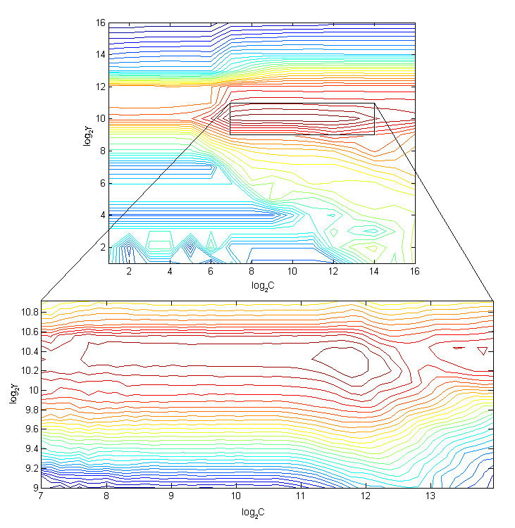
The guide from the authors of the LIBSVM library [35] recommends using exponentially growing sequence of parameters ( $C$ = $2^{-5}$ , $2^{-3}$ , $\dots$ , $2^{15}$ ; $\gamma$ = $2^{-15}$ , $2^{-13}$ , $\dots$ , $2^3$ ) in combination with the k-fold cross validation to find the optimal pair of the parameters. For bigger data sets, rough scale may be used for finding the best performing area of parameters on the grid at first. Then the finer grid resolution is applied to the best performing region. After finding the optimal ( $C$ , $\gamma$ ), the model should be retrained using the whole data set.

**Figure 6.** The example of the two-step grid search process is shown on this contour graph. Darker contours in red represent higher performance of the support vector machine on the testing data set. First, the region with highest performance is identified on the rough grid scale. Then the finer resolution is used to find the optimal parameter values. In this example, $C = 2^{11.8}$ , $\gamma = 2^{10.3}$ would be used to train the best performing SVM model.

**Figure 6.** The example of the two-step grid search process is shown on this contour graph. Darker contours in red represent higher performance of the support vector machine on the testing data set. First, the region with highest performance is identified on the rough grid scale. Then the finer resolution is used to find the optimal parameter values. In this example, $C = 2^{11.8}$ , $\gamma = 2^{10.3}$ would be used to train the best performing SVM model.

Missing values

Another problem that arises with the real world data sets are the missing values. This can be caused either by the fact, that some data were not collected from the beginning and started to be recorded at some later point. Or there might be some information that just could not be obtained from the applicant.

If such cases occur only rarely, we can just ignore those few incomplete points with a clear conscience. Naturally, a different approach must be taken if the missing values concern a big part of the total observations in the data set, as in such case it is not possible to simply disregard them.

For categorical variables, it is common among practitioners, that a new category “N/A” or “missing” is created. The other way how to deal with this problem is replacing the missing values with the mode value in its category. Missing values in numerical variables on the other hand can be replaced by the mean or median value.

While this technique may seem quite arbitrary on the first sight, it actually makes sense from the pragmatic point of view. Most of the learning algorithms cannot handle the data sets containing the missing values. If we still need to use such observations, it is best to assume, that the missing parts attain the most probable values. The real-world interpretation of this technique would be: if you do not know some information about the applicant, assume the most common value.

Feature selection

Many data sets contain a high number (hundreds, thousands or even much more in some study areas) of input features albeit only couple of them can be relevant to the examined classification problem. Credit scoring is not a typical example of high-dimensional problems, because there are rarely data sets containing more than like 100 input features in total.

Regardless, decreasing the dimensionality of the task can be beneficial both thanks to lower computational costs as well as increasing the performance of the resulting model. The irrelevant input features can actually bring additional noise into the model.

This is why some feature filtering or selection is often performed before the actual model training can begin. There are several established methods for this task, most of them are used in general and not limited only to the support vector machines context.

It should be noted, that feature selection techniques must be based on some kind of heuristic algorithms, since selecting the optimal set of the input features is not as simple job as it might seem at first sight. Suppose we have a data set with $n$ input features. Each of them can be found in one of the two possible states: included or not included in the final model. Thus there are $2^n$ possibilities to choose from.

The feature selection techniques are often combined with the model selection techniques. Each variant is then evaluated using the out-of-sample data set, which prevents to choose such features that perform well on the training subset (e.g. just by chance), but are not actually relevant to the classification task.

Forward selection

Forward selection is a sequential iterative procedure to select appropriate set of relevant input features. We start with an empty set of included features, i.e. all $n$ features are in the not included state at the beginning. Now we iterate over these features and use exactly one at a time, thus creating $n$ different models in the first step.

All these models are evaluated using the model selection procedure and the input feature performing best on the testing subset is chosen and included in the model.

In the next step, the remaining $n-1$ features produce a new set of $n-1$ models, each of them incorporating two input features – the one that was selected in the first step combined with one from the remaining features. Yet again the models’ performance is evaluated and the best performing feature is added to the set of included features.

This process goes on as long as it is necessary. In the support vector machines, there is no clear way how to decide, when the forward selection algorithm should stop. A researcher can for example set the reasonable amount of input features a priori. Or the stopping condition can be formulated as the minimum performance improvement required for each step. If in any given step the performance difference between the previous model and the new one is lower then some a priori set value, the Forward selection algorithm stops. The threshold value can either be zero (meaning to stop as soon as the newly added features start decreasing the performance of the model) or any other positive number.

Backward selection

The backward selection algorithm is a slight modification of the previous one. The main difference is that all of the input features are included in the model at the beginning. Then at each step, one worst performing feature is taken away in the same iterative manner. The stopping condition can be again some a priori chosen number of included input features or some performance threshold, as in the previous case.

Despite the fact, that forward and backward selection are essentially same, there are no guarantees that they end up with the same sets of the included input features.

F-score

A rather more quantitative and theoretically better justified approach to the feature selection is using of the F-score. Application of this method for the support vector machines was proposed by the LIBSVM authors in [10] and is used in many subsequent research papers on support vector machines in the credit scoring accordingly.

Given the training vectors $\vct{x}_k, k = 1,\dots,m$ , the number of positive and negative classes $m^+$ and $m^-$ , respectively, and the averages of the $i$ -th feature $\bar{x}_i$ , $\bar{x}_i^+$ , $\bar{x}_i^-$ , respectively, then the F-score of the $i$ -th input feature is defined by the following equation [10]:

(2) $\begin{equation*} F(i) = \frac{\left( \bar{x}_i^+ - \bar{x}_i \right)^2 + \left( \bar{x}_i^- - \bar{x}_i \right)^2} {\frac{1}{m^+ - 1} \sum_{k=1}^{n^+} \left( x_{k,i}^+ - \bar{x}_i^+ \right)^2 + \frac{1}{m^- - 1} \sum_{k=1}^{n^-} \left( x_{k,i}^- - \bar{x}_i^- \right)^2} \end{equation*}$

The higher the F-score the higher is the discriminative power of the respective attribute. The F-score is therefore a quite easily computable metric for judging the importance of each input feature although it has some drawbacks, too. The major disadvantage is that the F-score does not assess the relationships among the input features itself.

After the F-score is computed for all the input features some threshold has to be determined. Features with the F-score above this threshold will then be included in the model. The selection of the appropriate threshold can be done by iterating over some reasonable range of possible threshold values and minimizing the validation error of the corresponding models. [10]

Genetic algorithm

Genetic algorithms (GA) are biologically inspired optimization methods. They are very powerful in the optimization situations, where unattainable number of possibilities exist and the landscape of the problem is too complicated to use analytical solution.

Genetic algorithms mimic the process of the natural selection. The optimization problem must be translated in a suitable expression that plays the role of the DNA throughout the optimization – usually the binary encoding of the solution is used.

After that, some random set (i.e. population) from the set of all possible solutions is generated and evaluated. Subsequently, the best performing solutions are used to generate a new population through the combination of inheritance and several genetic operators: mutation and crossover. The process is repeated until some convergence criterion is met.

Although the genetic algorithms are not guaranteed to find a global extreme in all cases, it turns out that in many applications they are capable to find good enough solution in a satisfactory low number of steps. Concerned reader is referred to the relevant literature [26] for more information on this truly interesting topic.

In the association with the support vector machines, genetic algorithms are sometimes used for the feature selection. The problem is binary encoded in the chain of 0-1 numbers of length $n$ (the number of all features in the data set), whereas 0 representing the features that are not included and 1 representing the included features. E.g. for $m = 3$ , the chain $010$ represents a solution, where only 2nd feature is included in the model, while $111$ represents the model, where all features are considered relevant for the model.

A set of random chains is generated and the respective models are evaluated according to the model selection techniques. After the evolution is simulated in the sufficient number of steps, the chains representing near-optimal selection of input features will prevail in the entire population. Either the best performing model is directly chosen or the performance in combination with the number of features is taken into the consideration.

The experiments on the credit data sets show, that the genetic algorithms are effective for the feature selection, since they end up with as little as half of relevant features when compared to other techniques without sacrificing the performance of the models [36]. But the magic always comes with a price. In this case, the extreme requirements for the computer power represent such a cost.

Model selection

In practice, we have usually many model candidates to choose from and it may not be clear which one to use optimally for a given task. In the context of the support vector machines, the proper kernel function must be picked and then its optimal parameters found. Although most researchers use either linear or radial basis kernels for the credit scoring application, we need some general approach how to determine the optimal model from the class of all possibilities.

In principle, there are 3 basic methods that differ in the precision and the required computing resources.

Hold-out cross validation

The idea of this approach is rather simple: split the data set $S$ randomly into two subsets $S_{train}$ and $S_{test}$ , use only $S_{train}$ subset for training each model, and measure its performance on the $S_{test}$ subset. The model that performs best on $S_{test}$ is chosen as the optimal. Optionally, the selected model can be then retrained using the whole dataset $S$ in the end.

The advantage of the approach is low computational cost, while the disadvantage is that only the part of the dataset is used in the model selection process. This may be issue in cases, when the data is scarce or its acquisition was costly [46]. The split ratios 70:30 or 50:50 are most commonly used in the literature.

k-fold cross validation

During this process, dataset $S$ is randomly split into $k$ subsets $S_1,\dots,S_k$ . One of these subsets is left as a testing one and the rest $k-1$ are used to train the model. This process repeats $k$ times, so that each subset is left out as a testing one. Thus we obtain $k$ performance measures in the end. These measures are averaged for each model and the model with the best performance is chosen.

The advantage of the k-fold cross validation is more efficient use of the dataset, the disadvantage are higher computational costs since each model has to be trained $k$ times instead just once as in previous case. Usually, $k = 10$ or $k = 5$ are used in the literature as the default values. [46]

Leave-one-out cross validation

This is the special case of the previous approach when $k = m$ , i.e. each subset contains one observation. The computational costs are extreme so that the method can be used only on small datasets.

Model evaluation

When a best model is to be chosen from the set of several alternatives, a criterion to evaluate each model’s performance needs to be established. The simplified confusion matrix of the classification problem is given by Table 1.

		PREDICTED
		-1	+1
ACTUAL	-1	True Negative (TN)	False Positive (FP)
ACTUAL	+1	False Negative (FN)	True Positive (TP)

Table 1. The confusion matrix of the classification model. Each cell of the matrix contains a number of observations suiting the conditions in the respective heading. [42]

Simple criteria can be derived from this confusion matrix:

Accuracy (ACC) = $(TP+TN)/(TP+TN+FP+FN)$
Classification error = $(FP+FN)/(TP+TN+FP+FN)$
Sensitivity = $TP/(TP+FN)$ , also called true positive rate, hit rate or recall
Specificity = $TN/(FP+TN)$ , also called true negative rate

The support vectors machine algorithm leads to the separating hyperplane $(\vct{w}, b)$ which geometrically is, by default, positioned exactly in the middle between the support vectors of the $+1$ and $-1$ classes. Such treatment implicitly assumes that the negative consequences coming from the wrongly classified $+1$ class are of same seriousness as from the wrongly classified $-1$ class. This may not be always the case.²⁰

From his previous experience, the lender may know, that giving the loan to a bad creditor (falsely classified as a good one) is worse than missing the opportunity to fund a good creditor (falsely classified as a bad one). Such an information should be included in the model. To achieve this, we must shift the separating hyperplane closer to one or another class. Mathematically speaking, it means tweaking the parameter $b$ or, equivalently, changing the decision function so that the threshold score (2.42) for classification will be different from the default value 0.

In the logistic regression, this means to find a threshold $\tau$ other then the default value and then to classify an observation as $+1$ class when $P(Y=+1|\vct{x})>\tau$ and $-1$ otherwise.

The disadvantage of the metrics derived from the Table 1 rests in the fact that they represent a static picture, which is valid only for one choice of the threshold value.

A more sophisticated approach is represented by the Receiver Operating Characteristic (ROC) curve, which is a plot of the $Sensitivity$ on the y-axis against $(1-Specificity)$ on the x-axis across all possible thresholds. [42]

An aggregated single number, the area under the receiver operating characteristics curve (simply called as Area Under Curve or AUC), can be then calculated. AUC then serves as a metric for evaluating the model performance. The value of AUC = 0.5 corresponds to the random classification, while 1.0 indicates a perfect classification. An AUC is well-established in credit scoring and is explicitly mentioned in the Basel II accord. [42]

Formal statistical test has been developed by DeLong & DeLong to compare two or more areas under correlated ROC curves [18]. It can be used to test the hypothesis that the AUC of two different models (as measured on the same data set) is same. The method was later reformulated to the more accessible form in [21, p. 11] and applied specifically to the credit scoring problems.

Footnotes

²⁰ As an extreme example, consider the classification in medicine, where False positive test leads to emotional distress and the need for repeating the test while False negative can lead to the patient’s death.