2. Support vector machines – Support Vector Machines for Credit Scoring

Support vector machines present a unique combination of several key concepts [57]:

Maximum margin hyperplane to find a linear classifier through optimization
Kernel trick to expand up from linear classifier to a non-linear one
Soft-margin to cope with the noise in the data.

This chapter describes the derivation of the support vector machines as the maximum margin hyperplane using the Lagrangian function to find a global extreme of the problem. First, hard-margin SVM applicable only to linearly separable data is derived. Primal and dual form of the Lagrangian optimization problem is formulated. The reason, why the dual representation poses significant advantage for further generalization is explained. Further, a non-linear generalization using kernel functions is described and the “soft-margin” variation of algorithm, allowing for noise, errors and misclassification, is finally derived.

Maximum margin hyperplane

Let us start with the assumption, that the training data set is linearly separable. We are looking for the hyperplane parameters $(\vct{w}, b)$ , so that the distance between the hyperplane and the observations is maximized. We shall call the Euclidean distance between the point $\vct{x}_i$ and the hyperplane as geometric margin.

Definition 2.1. The geometric margin of an individual observation $\vct{x}_i$ is given by the equation

(1) $\begin{equation*} \delta_i = \frac{y_i ( \vct{w} \cdot \vct{x}_i + b )}{\|\vct{w}\|} \end{equation*}$

Note, that the equation (1) really does correspond to the perpendicular distance of the point,⁸ only the multiplier $y_i$ seems to be superfluous. But recall that $y_i$ assigns either +1 or -1. Its only purpose in the equation is to assure the distance to be a non-negative number. [44]

Definition 2.2. Given the training set D, the geometric margin of a hyperplane $(\vct{w},b)$ with respect to D is the smallest of the geometric margins on the individual training observations: [44]

(2) $\begin{equation*} \delta = \min_{i=1 \dots m} \delta_i \end{equation*}$

If we are looking for the optimal separating hyperplane, our goal should be to maximize the geometric margin of the training – i.e. to place the hyperplane such that its distance from the nearest points will be maximized. However, this is hard to do directly as such an optimization problem is a non-convex one. [44] Therefore, the problems needs to be reformulated before we can move forward.

Definition 2.3. The functional margin of an individual observation $\vct{x}_i$ is given by

(3) $\begin{equation*} \hat{\delta}_i = y_i ( \vct{w} \cdot \vct{x}_i + b ) \end{equation*}$

Definition 2.4. Given a training set D, the functional margin of $(\vct{w}, b )$ with respect to D is the smallest of the functional margins on the individual training observations. [44]

(4) $\begin{equation*} \hat{\delta} = \min_{i=1 \dots m} \hat{\delta}_i \end{equation*}$

Note, that there is a relationship between geometric margin and the functional margin:

(5) $\begin{equation*} \delta = \frac{\hat{\delta}}{\|\vct{w}\|} \end{equation*}$

Also note, that the geometric margin is scaling invariant – replacing the parameters $(\vct{w}, b )$ with $(2 \vct{w}, 2 b )$ , for instance, will not change the results. The opposite is true for the functional margin. Therefore we may impose an arbitrary scaling constraint on $\vct{w}$ conveniently to suit our needs. We will set the scaling so that the functional margin is 1 and maximize the geometric margin under this constraint. [44]

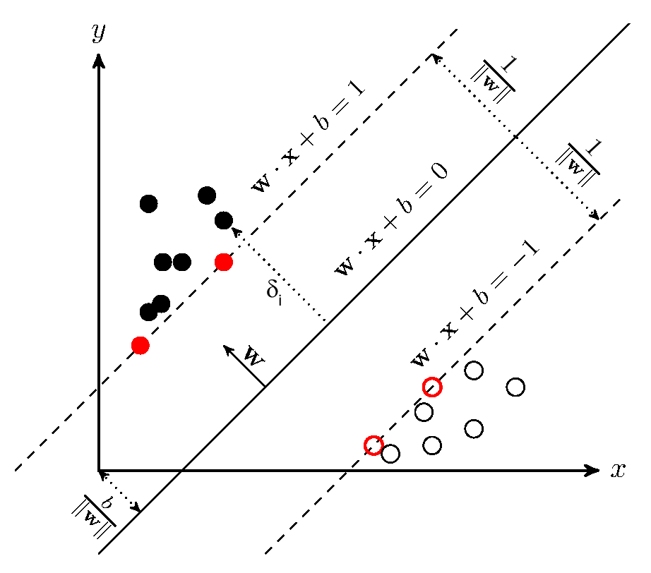(6) $\begin{equation*} \hat{\delta} = 1, \end{equation*}$

**Figure 3.** Geometric margin and maximum margin hyperplane (line in 2-D). The solid line separates two classes (filled and empty circles) and is fully defined by the vector of weights $\vct{w}$ which is perpendicular to the line and bias $b$ , which determines the position of the line with respect to the origin. The distance between each point and the line is called geometric margin $\delta_i$ and defined in (1). There will always be some points that are closest to the line (marked red). Using the appropriate scaling (6), their distance can be set to $\frac{1}{\| \vct{w} \|}$ . In further steps, the goal is to maximize this distance. Credits: Yifan Peng, 2013 [49].

When we want to maximize the geometric margin, from (5) it follows that we need to maximize the term $\frac{1}{\| \vct{w} \|}$ . Such a task is equal to the minimization of $\| \vct{w} \|$ in the denominator. Yet this task is still quite a difficult one to solve, as by (1.1) it would involve the terms in a square root.

Nevertheless, it is possible to replace this term by $\frac{1}{2}\| w \|^2$ without changing the optimal solution.⁹ The multiplier $\frac{1}{2}$ is added for the mathematical convenience in later steps and again, does not affect the position of the extreme.

Finally, applying (1.3), the objective function to be minimized is

(7) $\begin{equation*} \Phi(\vct{w},b) = \frac{1}{2} \ \vct{w} \cdot \vct{w} \end{equation*}$

It is necessary to ensure that the equation (4) holds when the objective function is minimized. The functional margin of each individual observation must be equal to or larger than the functional margin of the whole dataset.

(8) $\begin{equation*} y_i ( \vct{w} \cdot \vct{x}_i + b ) \geq \hat{\delta}, \ \forall i \end{equation*}$

By substituting (6), we have

(9) $\begin{equation*} y_i ( \vct{w} \cdot \vct{x}_i + b ) \geq 1, \ \forall i \end{equation*}$

This inequality poses a constraint to the optimization problem (7). [44]

The solution of this problem will be a linear decision surface with the maximum possible margin (given the training dataset). The objective function is clearly a convex function which implies that we are able to find its global maximum. The entire optimization problem consists of a quadratic objective function (7) and linear constraints (9) and is therefore solvable directly by the means of the quadratic programming. [28, p. 82]

Lagrangian methods for optimization

Since the means of the quadratic programming are usually computationally inefficient when dealing with large data sets¹⁰, we will continue solving this optimization problem using the Lagrangian methods.¹¹

Let us start more generally and then apply the mathematical theory to the problem of finding the maximum-margin hyperplane.

Primal problem

Consider the optimization problem

(10) $\begin{eqnarray*} \begin{aligned} & \min_{\vct{w}} & & f(\vct{w}) \\ & s.t. & & g_i(\vct{w}) \leq 0\\ &&& h_i(\vct{w}) = 0 \end{aligned} \end{eqnarray*}$

The minimization is constrained by an arbitrary number of equality and inequality constraints.¹² One method to solve such a problem consists in formulating a derivative problem, that has the same solution as the original one. Define the generalized Lagrangian function of (10) as

(11) $\begin{equation*} \mathcal{L}( \vct{w}, \alpha, \beta ) = f(\vct{w}) + \sum_i \alpha_i g_i(\vct{w}) + \sum_i \beta_i h_i(\vct{w}) \end{equation*}$

Further define

(12) $\begin{equation*} \theta_P(\vct{w}) = \max_{\alpha,\beta;\alpha_i\geq0} \mathcal{L}(\vct{w},\alpha,\beta) \end{equation*}$

This allows as to formulate the so called primal optimization problem, denoted by subscript $P$ on that account:

(13) $\begin{equation*} p^* = \min_{\vct{w}} \theta_P(\vct{w}) = \min_{\vct{w}} \max_{\alpha,\beta;\alpha_i\geq0} \mathcal{L}(\vct{w},\alpha,\beta) \end{equation*}$

Note that the function $\theta_P$ value assumes plus infinity, in case any constraint from (10) does not hold. If $g_i(\vct{w}) > 0$ for any $i$ , (12) can be maximized by simply setting $\alpha = +\infty$ . If on the other hand $h_i(\vct{w}) \neq 0$ , (12) is maximized by setting $\beta$ to plus or minus infinity (depending on the sign of the function $h_i$ ).

If all the constraints hold, $\theta_P$ takes the same value as the objective function in the original problem, $f(\vct{w})$ . Provided both constraints hold, the third equation term in (11) is always zero and the second term is also maximized when it is set to zero by appropriate setting of weights $\alpha_i$ . Thus we have

(14) $\begin{equation*} \theta_P(\vct{w}) = \begin{cases} f(\vct{w}) & \text{if constraints are satisfied}\\ +\infty & \text{otherwise} \end{cases} \end{equation*}$

It is obvious that (13) is, indeed, equal to the original problem (10).

Dual problem

We could solve the primal problem, but when applied to our task, the properties of the algorithm would not bring much benefits. Instead, for the sake of the forthcoming solutions, let us define a different optimization problem by switching the order of minimization and maximization.

(15) $\begin{equation*} \theta_D(\alpha,\beta) = \min_{\vct{w}} \mathcal{L}(\vct{w},\alpha,\beta) \end{equation*}$

The subscript $D$ stands for dual and it will be be used to formulate the so called dual optimization problem:

(16) $\begin{equation*} d^* = \max_{\alpha,\beta;\alpha_i \geq 0} \min_{\vct{w}} \mathcal{L} ( \vct{w}, \alpha, \beta ) = \max_{\alpha,\beta} \theta_D \end{equation*}$

The value of the primal problem $p^*$ and the dual problem $d^*$ is not necessarily equal. There is a generally valid relationship between maximum of minimization and minimum of maximization

(17) $\begin{equation*} d^* \leq p^* \end{equation*}$

The difference between primal and dual solution, $p^* - d^*$ is called the duality gap. As follows from (17), the duality gap is always greater than or equal to zero.

Certain conditions have been formulated that (if met) guarantee the duality gap to be zero, i.e. under such conditions, the solution of the dual problem equals to the solution of the primal one.

Definition 2.5. Suppose $f$ and all functions $g_i$ are convex and all $h_i$ are affine. Suppose that the constraints are strictly feasible (i.e. there exists some $\vct{w}$ so that $g_i(\vct{w}) < 0$ for all $i$ ). Then there exist $\vct{w}^*$ , $\alpha^*$ , $\beta^*$ so that $\vct{w}^*$ is the solution to the primal problem, $\alpha^*$ , $\beta^*$ is the solution to the dual problem, $p^* = d^* = \mathcal{L}( \vct{w}^*, \alpha^*, \beta^* )$ and $\vct{w}^*, \alpha^*, \beta^*$ satisfy following Karush-Kuhn-Tucker (KKT) conditions [44]

(18) $\begin{equation*} \frac{\partial \mathcal{L}}{\partial w_i}\ =\ 0,\ & \ i = 1,\dots,n\\ \end{equation*}$

(19) $\begin{equation*} \frac{\partial \mathcal{L}}{\partial \beta_i}\ =\ 0,\ & \ i = 1,\dots,n\\ \end{equation*}$

(20) $\begin{equation*} \alpha_i^*g_i(\vct{w}^*)\ =\ 0,\ & \ i = 1,\dots,n\\ \end{equation*}$

(21) $\begin{equation*} g_i(\vct{w}^*)\ \leq\ 0,\ & \ i = 1,\dots,n\\ \end{equation*}$

(22) $\begin{equation*} \alpha_i^*\ \geq\ 0,\ & \ i = 1,\dots,n \end{equation*}$

Remark: For its specific importance, KKT condition (20) is often referred as complementary condition.

Application to maximum margin hyperplane

Let us return to our original task defined by equations (7), (9). The constraint can be rewritten in order to match the form of (10)¹³

(23) $\begin{equation*} g_i(\vct{w}) = - y_i( \vct{w} \cdot \vct{x}_i + b ) + 1 \leq 0 \end{equation*}$

The Lagrangian of the objective function (7) subject to (9) will be, according to (11)

(24) $\begin{equation*} \mathcal{L}(\vct{w}, \vct{\alpha}, b) = \frac{1}{2} \vct{w} \cdot \vct{w} - \sum_{i=1}^m \alpha_i \left( y_i ( \vct{w} \cdot \vct{x}_i + b ) - 1 \right) \end{equation*}$

The dual can be found quite easily. To do this, we need to first minimize $\mathcal{L}$ . [44] By (18) we take the partial derivatives of $\mathcal{L}$ with respect to $\vct{w}$ and $b$

(25) $\begin{equation*} \vct{w} &= \sum_{i=1}^m \alpha_i y_i x_i\\ \end{equation*}$

(26) $\begin{equation*} \sum_{i=1}^m \alpha_i y_i &= 0 \end{equation*}$

Substituting these equations into (24) and simplifying the result

(27) $\begin{equation*} \mathcal{L}(\vct{w},\vct{\alpha},b) = \sum_{i=1}^m \alpha_i - \frac{1}{2} \sum_{i=1}^m \sum_{j=1}^m \alpha_i \alpha_j y_i y_j \ \vct{x}_i \cdot \vct{x}_j \end{equation*}$

This equation was obtained by minimizing $\mathcal{L}$ with respect to $\vct{w}$ and $b$ . [44] According to (16), this expression needs to be maximized now. Putting it together with (22) and (26), the dual optimization problem is

(28) $\begin{eqnarray*} \begin{aligned} & \max_{\vct{\alpha}} & & \left( \sum_{i=1}^m \alpha_i - \frac{1}{2} \sum_{i=1}^m \sum_{j=1}^m \alpha_i \alpha_j y_i y_j \ \vct{x}_i \cdot \vct{x}_j \right) \\ & s.t. & & \sum_{i=1}^m \alpha_i y_i = 0\\ & & & \alpha_i \geq 0, \ i = 1,\dots,l \end{aligned} \end{eqnarray*}$

It can be shown, that KKT conditions are met and that (28) really presents a solution to the original problem. [28]

One interesting property should be pointed out at the moment. The constraint (9) actually enforces the fact that the functional margin of each observation should be equal to or greater than the functional margin of the dataset (which we set by (6) to one).

It will be exactly one only for the points closest to the separating hyperplane. All other points will lie further and therefore their functional margin will be higher than one. By the complementary condition (20) the corresponding Lagrangian multipliers $\alpha_i$ for such points must be equal to zero. [14, p. 97]

Therefore the solution of the problem, the weight vector $\vct{w}$ in (25), depends only on a few points with non-zero $\alpha_i$ that lie closest to the separating hyperplane. These points are called support vectors. [14, p. 97]

The solution of the dual problem (28) leads to an optimal vector $\vct{\alpha}^*$ , which can be immediately used to calculate the weight vector of the separating hyperplane $\vct{w}$ using (25). Since most of the $\alpha_i$ coefficients will be zero, the weight vector will be a linear combination of just a few support vectors.

Having calculated the optimal $\vct{w}^*$ , the bias $b^*$ must be found making use of the primal constraints, because the value $b$ does not appear in the dual problem: [14, p. 96]

(29) $\begin{equation*} b^* = -\frac{\max_{y_i=-1} \vct{w}^* \cdot x_i + \min_{y_i=+1} \vct{w}^* \cdot x_i}{2} \end{equation*}$

From (1.9) this leads to a decision function that can be used to classify new out-of-sample observation $\vct{x}$ :

(30) $\begin{equation*} \hat{f}(\vct{x}) = sgn \left( \sum_{i=1}^m \alpha_i^* y_i \vct{x}_i \cdot \vct{x} - b^* \right) \end{equation*}$

As stated above, this classifier is determined completely only by the support vectors. Because of this property, it is called a support vector machine. To be more precise, a linear support vector machine, since it is based on a linear decision surface. [28, p. 102] It is able to classify linearly separable data only. On the other hand, unlike some other classifiers, it is guaranteed to converge and find the hyperplane with the maximum margin. Since the optimization problem is a convex and KKT conditions are met, there is always a unique solution and it is a global extreme.¹⁴

There is one remarkable property in the decision function (30) that is worthy of our special attention. The observations only appear there as dot products between the input vectors. This opens a door to the use of a special technique that researcher usually refer as “kernel trick”. Owing to it, the linear support vector machine derived in this section can be extended and generalized to fit almost any non-linear decision surface.

Kernels and kernel trick

The problem with the real life data sets is that the relationship among the input variables are rarely simple and linear. In most cases some non-linear decision surface would be necessary to correctly separate the observations into two groups. This necessity, on the other hand, noticeably increases the complexity and computational difficulty of such a task.

Instead, the support vector machines implement another conceptual idea: the input vectors are mapped from an original input space into a high-dimensional feature space through some non-linear mapping function chosen a priori. The linear decision surface is then constructed in this feature space. [12]

The underlying justification can be found in Cover’s theorem [13], which may be qualitatively expressed as:

A complex pattern-classification problem, cast in a high-dimensional space nonlinearly, is more likely to be linearly separable than in a low-dimensional space, provided that the space is not densely populated. [34, p. 231]

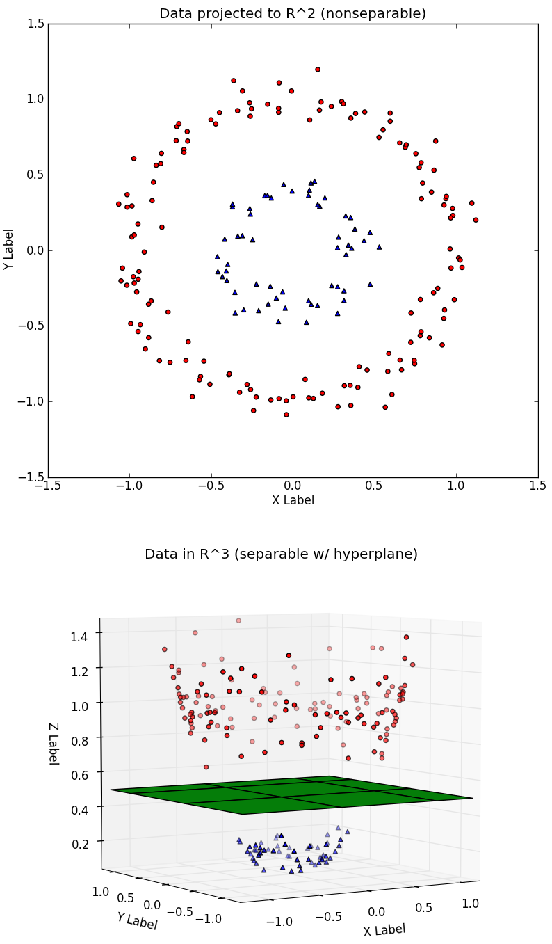
**Figure 4.** An example of the data set, that is not linearly separable in the original space $\mathbb{R}^2$ (Top). The very same data set can be however separated linearly in the transformed space obtained by the transformation: $[x_1, x_2] = [x_1,x_2, x_1^2 + x_2^2]$ (Bottom). Credits: Eric Kim, 2013 [39].

Because now we want to operate in the feature space rather than in the original input space, we can slightly modify the original equation (28) and replace the plain dot products $\vct{x}_i \cdot \vct{x}_j$ with $\phi( \vct{x}_i ) \cdot \phi( \vct{x}_j )$ . By $\phi(\cdot)$ we denote some appropriately chosen mapping function.

Consider that the transformation $\phi(\vct{x})$ may be very complex, complicated. The results could belong to high dimensional, in some cases even infinitely dimensional spaces. Such transformations would be computationally very expensive or even impossible to do.

The key idea of this concept is contained in the fact, that to find the maximum margin hyperplane in the feature space, one actually need not to calculate the transformed vectors $\phi(\vct{x_i}), \phi(\vct{x_j})$ explicitly, since it is present only as a dot product in the training algorithm.

It would be very wasteful to spend a precious computational time to perform these complex transformations only to aggregate them immediately in a dot product, one single number.

It appears that for our needs it is sufficient to use a so called kernel function which is defined as a dot product of the two transformed vectors and which may be calculated very inexpensively. [44]

Definition 2.6. Given an appropriate mapping $\phi: \mathbb{R}^n \rightarrow \mathbb{R}^m$ with $m \geq n$ , the functions of the form

(31) $\begin{equation*} K( \vct{x}, \vct{z} ) = \phi( \vct{x} ) \cdot \phi( \vct{z} ) \end{equation*}$

where $\vct{x}, \vct{z} \in \mathbb{R}^n$ are called kernel functions or just kernels. [28, p. 107]

The process of mapping the data from the original input space to the feature space is called kernel trick. [28, p. 103] The kernel trick is rather universal approach, its application is not solely limited to the support vector machines. In general, any classifier that depends merely on the dot products of the input data may capitalize on this technique.

Let us rephrase the support vector machines using the kernel functions. The training algorithm 28 can be now expressed as

(32) $\begin{eqnarray*} \begin{aligned} & \vct{\alpha}^* = \argmax_{\vct{\alpha}} & & \sum_{i=1}^m \alpha_i - \frac{1}{2} \sum_{i=1}^m \sum_{j=1}^m \alpha_i \alpha_j y_i y_j K( \vct{x}_i, \vct{x}_j ) \\ & s.t. & & \sum_{i=1}^m \alpha_i y_i = 0\\ & & & \alpha_i \geq 0, \ i = 1,\dots,l \end{aligned} \end{eqnarray*}$

while the decision surface (30) in terms of kernel function is defined as

(33) $\begin{equation*} \hat{f}(\vct{x}) = sgn \left( \sum_{i=1}^m \alpha_i^* y_i K( \vct{x}_i, \vct{x}) - b^* \right) \end{equation*}$

Linear kernel

There are several well known kernel functions that are commonly used in connection with support vector machines.

The first, rather trivial, example is a linear kernel. It is defined simply as

(34) $\begin{equation*} K(\vct{x},\vct{z}) = \phi(\vct{x}) \cdot \phi(\vct{z}) = \vct{x} \cdot \vct{z} \end{equation*}$

In this case, the feature space and the input space are same and we get back to the solution derived in the previous Section, where we discussed linear support vector machines.

I mention the linear kernel here just to emphasize the fact, that the substitution with the kernel function does not change the original algorithm entirely. It merely generalizes it.

Polynomial kernel

The polynomial kernels are another example of frequently used kernel functions. When Vapnik and Cortes in their essential paper [12] achieved a great shift in the optical character recognition of handwritten numbers, it was the polynomial kernel that showed its strength for this particular task.

The homogeneous polynomial kernel of degree $d$ ( $d \geq 2$ ) is defined as

(35) $\begin{equation*} K(\vct{x},\vct{z}) = ( \vct{x} \cdot \vct{z} ) ^ d \end{equation*}$

The more general non-homogeneous polynomial kernel ( $d \geq 2, c > 0$ ) is

(36) $\begin{equation*} K(\vct{x},\vct{z}) = ( \vct{x} \cdot \vct{z} + c ) ^ d \end{equation*}$

Note, that the latter maps the original input space to the feature space of the dimensionality $\binom{n+d}{d}$ , where $d$ is the degree of the kernel and $n$ is the dimension of the original input space. However, despite working in this $O(n^d)$ -dimensional space, computation of $K(\vct{x},\vct{z})$ consumes only $O(n)$ time. [44]

Gaussian kernel (Radial basis function)

The gaussian kernel is probably the mostly used kernel function and is defined as

(37) $\begin{equation*} K(\vct{x},\vct{z}) = exp \ \left\{ - \frac{\| \vct{x} - \vct{z} \|^2}{2 \sigma^2} \right\} \end{equation*}$

It maps the input space to the infinitely dimensional feature space. Thanks to this property, it is very flexible and is able to fit a tremendous variety of shapes of the decision border. The gaussian kernel is also often referred as radial basis function (RBF). In some instances is parametrized in a slightly different manner:

(38) $\begin{equation*} K(\vct{x},\vct{z}) = exp \ \left\{ - \gamma \| \vct{x} - \vct{z} \|^2 \right\} \end{equation*}$

Other kernels

There are many other well researched kernel functions. An extensive, although probably not exhaustive, list of other commonly used kernel functions is available in [17]. Most of them are, however, used only for research purposes or under the special circumstances and have no use in the credit scoring models.

For any function K to be a valid kernel, a necessary and sufficient condition has been derived. This condition is usually referred as Mercer’s theorem, which is formulated in a slightly simplified form below [44].

Definition 2.7. Let a finite set of $m$ points be given $\left\{ x_1,\dots,x_m \right\}$ and let a square $m$ -by- $m$ matrix $K$ be defined so that $(i,j)$ entry is given by $K_{ij} = K(x_i,x_j)$ . Then such a matrix is called Kernel matrix.

Theorem 2.1. (Mercer’s theorem)
Let $K : \mathbb{R}^n \times \mathbb{R}^n \rightarrow \mathbb{R}$ be given. Then for $K$ to be a valid kernel, it is necessary and sufficient that for any $\left\{ x_1, \dots x_m \right\}, m < \infty$ , the corresponding kernel matrix is symmetric positive semi-definite.

There are no general rules concerning the selection of a suitable kernel. It highly depends on the character of the task being solved, the data set and the relationships among the variables play a major role, too. In case of simple jobs with plain linear relationships, the linear kernel may be sufficient and other kernels will not bring any improvement.

In other applications, where the data are complex and interdependent, more advanced kernels may bring a major leap in the classification performance. This may be the case in the aforementioned optical character recognition (OCR), face recognition, natural language processing or genetics.

The credit scoring lies kind of in the middle of these extremes. Some papers suggest, that the consumer credit scoring data tend to be linear or just mildly non-linear. Therefore, the linear support vector machines predominate in the literature, often accompanied with the Gaussian kernel to seek for the non-linearities in the data (see [42] for comprehensive list of papers). The polynomial kernels are rarely represented in the credit scoring literature (see [5], [56] for examples) as they seem to give the mixed results.

Soft margin classifiers

Until now we have assumed that our training data are linearly separable – either directly in the input space or in the feature space. In other words we have supposed only perfect data sets. In reality the data sets are often far from perfect. The real data are noisy, contain misclassified observations, random errors etc.

We need to generalize the algorithm to be able to deal with the non-separable data. Surprisingly enough, the basic idea of the generalization is very simple. We just need to allow some observations to end up on the “wrong” side of the separating hyperplane.

The required property is accomplished by introducing a slack variable $\xi$ and rephrasing the original constraint (9)

(39) $\begin{equation*} y_i ( \vct{w} \cdot \vct{x}_i + b ) \geq 1 - \xi_i, \ i=1,\dots,l \end{equation*}$

where $\xi_i \geq 0$ . This way we allow the functional margin of some observations to be less than 1.

The slack variable works like a corrective equation term here. For the observations located on the correct side of the hyperplane, the respective $\xi_i = 0$ and the (39) is then same as (9). For noisy or misclassified observations appearing on the wrong side of the hyperplane, the respective $\xi_i > 0$ , as shown in Figure 5.

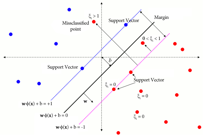
**Figure 5.** The purpose of the slack variable explained through the simple sketch. The respective slack variable $\xi_i$ is zero if the observation is located on the correct side of the hyperplane and nothing is changed. The $\xi_i$ is greater than zero if its distance from the separating hyperplane is lower than the distance of support vectors. Credits: Stephen Cronin, 2010, slightly modified. [15] .

It is necessary that with each misclassification we pay some price, since in general we want to maximize the margin while simultaneously minimize the adverse effect of the wrong observations. Otherwise the trivial solutions where all data are marked as wrong would always prevail. This is why we have to expand the original objective function by the penalty term

(40) $\begin{equation*} \min_{\vct{w},\vct{\xi},b} \left( \frac{1}{2} \vct{w} \cdot \vct{w} + C \sum_{i=1}^m \xi_i \right) \end{equation*}$

where $C > 0$ is the cost parameter, which determines the importance of wrong observations. Small values of C lead to more benevolent solutions while the larger values of C would lead to solutions similar to the hard margin classifier from the previous sections.

This time due to the limited space I will not go again through the whole process of deriving the dual of this problem (for the step by step solution see [28, p. 118-121]. It turns out, that the dual of the soft margin classifier simplifies to a very convenient form:

(41) $\begin{eqnarray*} \begin{aligned} & \max_{\vct{\alpha}} & & \left( \sum_{i=1}^m \alpha_i - \frac{1}{2} \sum_{i=1}^m \sum_{j=1}^m \alpha_i \alpha_j y_i y_j K( \vct{x}_i, \vct{x}_j ) \right) \\ & s.t. & & \sum_{i=1}^m \alpha_i y_i = 0\\ & & & C \geq \alpha_i \geq 0, & i = 1,\dots,l \end{aligned} \end{eqnarray*}$

Note that the newly inserted cost term does not appear in the objective function and poses only a restriction for the values of the individual $\alpha$ coefficients.

Thanks to this property and combined with the kernel trick, the soft margin support vector machines are very easily implemented and solved efficiently on the computers without requiring a tremendous computational power.

The results, again, will be the decision function (30). This function produces results on the simple yes/no scale. In credit scoring we often need more than that: we need to quantify the quality of the debtor as a real-valued number which is then called score in this context. This may come handy in tasks like calculating the area under curve or finding the optimal cut-off value, which both will be discussed later in the text.

For this purpose, the functional margin of the observation can be used. Thus, the score $s$ of the observation $\vct{x}$ will be simply defined as

(42) $\begin{equation*} s(\vct{x}) = \sum_{i=1}^m \alpha_i^* y_i \vct{x}_i \cdot \vct{x} - b^* \end{equation*}$

where $\vct{\alpha}^*$ , $b^*$ are the parameters of the optimal hyperplane calculated by the support vector machines, $\vct{x}_i$ , $y_i$ are the individual observations from the training set and $m$ is the number of observations in the training data set.

Algorithm implementation

The simplest approach to solve a convex optimization problem numerically on computers is the gradient ascent, sometimes known as the steepest ascent algorithm. The method starts at some arbitrary initial vector (e.g. rough estimate of the possible solution) and proceeds iteratively, updating the vector in each step in the direction of the gradient of the objective function at the point of the current solution estimate. [14, p. 129]

But using the gradient methods to solve (41) brings problems which are hard to be circumvented. The main trouble is caused by the fact, that the constraint $\sum_{i=1}^m \alpha_i y_i = 0$ must hold on every iteration. From this constraint it follows, that the elements of vector of solutions, $\vct{\alpha}$ are interconnected and cannot be updated independently. It also implies, that the smallest number of multipliers that can be optimised at each step is 2. [14, p. 137]

This key fact is used by the algorithm Sequential Minimal Optimisation (SMO) which, in the course of time, was established as the optimal way to solve the problem (41). At each iteration, the SMO algorithm chooses exactly 2 elements of the optimised vector, $\alpha_i$ and $\alpha_j$ , finds the optimal values for those elements given that all others are fixed and updates the vector $\vct{\alpha}$ accordingly. [14, p. 137]

In each step, the vector $\alpha_i$ and $\alpha_j$ are chosen by the heuristics described in [50] by Platt, who first introduced the SMO algorithm; the optimisation itself is however solved analytically in every iteration. The introduction of SMO removed the main barrier for support vector machines to be widely adopted by the researchers, as it sped up the training process at least 30 times against the methods used before. [19]

Since then, the SMO efficiency was further improved and it quickly became a standard for the support vector machines training.

Because of the fact, that the actual process of implementation of the training algorithm is rather tedious, prone to errors and represents more just a technicality rather than actual research value, the standardized packages and libraries to support the SVM training and evaluation were created.

Among them, LIBSVM [9] is the most prominent one, with the longest history, continuous updates, associated research paper and data sets and widest support for different development environments (IDEs). Other libraries, like SVMlight¹⁵, mySVM¹⁶ or the specialised toolbox for R¹⁷, Torch¹⁸ or Weka¹⁹ do exist.

Matlab, which was used for the practical part of my thesis, has its own support for SVM. However, its performance and the possibilities it offers are not astonishing. For that reason, I decided to use the LIBSVM library as an extension for the standard Matlab functions.

Footnotes

⁸ See [48, p. 161] for details and proof.

⁹ Optimization over the positive values $\| \vct{w} \|$ is invariant under the transformation with the square function. In general, $x^2$ is a monotonic function for $x \geq 0$ . Therefore optimizing over $x^2$ is same as optimizing over $x$ . [28, p. 81]

¹⁰ thousands or tens of thousands of observations

¹¹ This whole section of my work is based mostly on the online videolecture of professor Andrew Ng from the Stanford University [45] who (along with many other lecturers from the most prominent universities) made his knowledge freely available under the Creative Commons license to people from all over the world. For that I express him (them) my deepest gratitude.

¹² Note, that (10) embodies a very broad class of problems. For example, any maximization problem can be transformed to the minimization, since $\max x = \min -x$ or $\max x = \min \frac{1}{x}$ , if defined. Also any constrained in the form $g(x) \geq 0$ can be converted to the form of (10) multiplying by (-1) and every constraint in the form $h(x) = b$ can be transformed by subtracting $b$ to the desirable form.

¹³ Note, that there are no equality constraints in this task, so there will be no $h_i$ terms.

¹⁴ Even some advanced classification algorithms, like neural networks, must face the problem that they may get “stuck” in the local extreme and find only a suboptimal solution.

¹⁵ http://svmlight.joachims.org/

¹⁶ http://www-ai.cs.uni-dortmund.de/SOFTWARE/MYSVM/index.html

¹⁷ SVM in R, http://cran.r-project.org/src/contrib/Descriptions/e1071.html

¹⁸ SVMTorch, http://www.idiap.ch/learning/SVMTorch.html

¹⁹ http://www.cs.waikato.ac.nz/ml/weka/